
Gun Violence in America : An Analysis

Quick Links:
- Background
- The Data
- How do Gun Murder Rates Vary Across States through Time?
- Does Month Affect Murder Patterns?
- Which States are Best at Solving Murders?
- Which Cities are Getting Better at Solving Murders?
- Does Victim Race Affect Whether a Murder is Solved?
- Can We Predict the Age of a Killer?
- How about Predicting Whether a Crime will be Solved or Not?
- Conclusions
- References
Background

Gun violence has become an epidemic in the United States in recent years. In 2017 alone, there have been over 4500 gun related deaths in the U.S. so far. With this epidemic has come fervent discussion from those who wish to relax gun controls and those who wish to strengthen them. Indeed, this issue of gun control has latched itself onto American politics, ideology, and identity in a way unlike any other nation. The key question is of course: What should the U.S. do about it? Should we adopt more restrictive policies mirroring countries like Germany, the UK, and Italy? Or should we place fewer limits on who can purchase a gun, rationalized by the idea that Americans are free to protect themselves?
Still, these are not the most pressing questions when it comes to gun violence in America. Before we can take real steps towards eradicating deaths by firearms, we need to understand the underlying dynamics. Before we can figure out how to reduce deaths by guns, we need to figure out which groups are suffering most from gun related deaths, whether by race, sex, or geographic region. Before we can figure out how to better solve gun related crimes, we need to understand how good we are at solving them, at the national, state, and county level. Before we can better protect against gun violence, we need to determine when gun violence is most likely to be high.
We will explore all these questions through this post. We will spend the latter part of the post going one step further and using techniques in machine learning to predict the age of a killer in cases when we have no leads and whether or not a crime will be solved at all. Besides being very applicable in predictive policing, we can analyze the most predictive features in our models to further understand the dynamics at play in the American gun violence epidemic.
The Data
The data for this analysis came from an FBI dataset on homicides in the United States from 1980 to 2014. This dataset includes not only gun murders but murders from other methods as well including knives, drowning, fire, drugs, etc. We will focus only on the gun murders for this study. Note that gun murders account for 66% of all homicides from 1980 to 2014.
The data includes information about the county and state in which the murder occurred, the month and year it occurred, a field indicating whether or not the crime was solved, information about the victim and perpetrator including sex, race, ethnicity, age, the weapon used in the murder, and finally the relationship between the perpetrator and victim, if any.
There are a few notes to be made about the data to ensure a better understanding of the following analysis. First, note that we often do not have the perpetrator information. This is surely true if the crime was not solved since we do not know who the killer was but we also sometimes have missing information even when the crime was solved. This is the motivation behind the latter part of this post when we try and predict whether or not a crime will be solved and the age of the killer.
Without further ado, let us dive in!
How do Gun Murder Rates Vary Across States through Time?
One natural question we can ask is how serious of a problem gun violence is. That is, how many people lose their lives to gun related crimes and does this number vary by state and over time between 1980 and now? We choose some the most populous U.S. states, California, Illinois, Texas, New York, as well as Arizona for some particularities in its trend which we’ll see. For each of these states, as well as for the United States as a whole, we plot the number of gun murders each month from 1980 to 2014, scaled by the population of that state. This scaling is important since a more populous state will likely have more gun murders.
We take our state population data from the U.S. Census Bureau, which collects population information every ten years. That is, we use the years 1980, 1990, 2000, and 2010 for this information, and assume a constant population in between. This is not completely true but it’s the best we can do here.
Feel free to toggle, click, and hover over the individual states below!
Gun Murders per Month Scaled by Population (per 1,000,000 residents)
Here are a few key takeaways:
- The rate of gun violence has in general gone down from 1980 until now. Looking a bit deeper, we see that in the early 90s, there was a peak in gun related deaths overall as well as for many states including California, New York, and Texas. A bit of good news here in terms of the overall trend over time.
- The volatility of gun related deaths has also gone down over time. that is, the individual state lines, as well as the national line to an extent, have become less sporadic over time. This might be partly explained by increasing populations in most states and nationally. That is, when there are more people in a state, the true trend of gun related deaths is more clear and subject to less noise. You can even see that just by comparing states! Look at the low volatility of extremely populous California compared to the extreme jumpiness of Arizona, six times less populous.
- We also see evidence of ‘convergence’ going on. That is, around 1980 to 2000, the states, as we noted, were very volatile and showed only weak correlation as a whole. But, after 2000, we see that the states seem to ‘converge’ around 3 deaths per 1000000 residents.
Let’s zoom in on that post 2000 range to get a better look at recent trends!
Gun Murders per Month Scaled by Population (per 1,000,000 residents)
- Looking at this closer level we can clearly see the structures and cycles. Looking first at the national line, we see a strong recurring trend that the peaks when there is the most gun violence occur in July and the dips when there is the least gun violence, occurs in February of each year. Keep those months in mind, we’ll see some extra evidence to back it up soon.
- Looking at Arizona, we see abnormally high values for gun related deaths in recent years with the highest point being 8 deaths per 1000000 residents in May of 2002.
- We also see that Illinois continues to be very volatile, going against our hypothesis that more populous states should in general have lower volatilities due to the high sample size negating the noise.
We turn our attention next to monthly differences in gun murders across all states.
Does Month Affect Murder Patterns?
We have looked at data so far by month and state, but let us take a step back now and look at montly trends regardless of state. We will answer two questions.
The first question we ask is how occurrences of gun murders change by month. In which months do the most deaths occur? The least? Note that for the following two bar graphs, we look at data from 2000 and beyond in order to understand the most recent trends.
Let’s turn to the data!
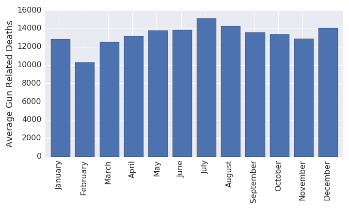
- We see immediately that the most murders occur in July and the least in February, as indicated by the previous section, but deeper than that we see that there are two peaks in the year and two dips. The other peak occurs at December and the other dip occurs just before, in November.
- It should not be too surprising that there are the fewest gun related deaths in February. February has at least one less day than any other months, sometimes two or three fewer. With fewer days, as with a small population, comes fewer murders.
- And what about the peak in July? It is a commonly known phenomenon that crime including gun murder goes up significantly on the Fourth of July. If we had time data at the day level, we could remove the fourth of each month and recompute the monthly means in gun related deaths and see if July is still a peak.
We turn away from the occurrences of gun deaths in the U.S. and towards the accuracy in solving gun deaths, catching the killer, based on county, state, time period, etc. We want to know just how good we are as a people at solving gun murders, and stopping killers from killing again. We also want to know if we have any biases at the national and state levels in catching a killer based on whether the victim is Black, White, Asian, Native American, etc.
Let’s start simple. How good are we at solving gun murders by month?
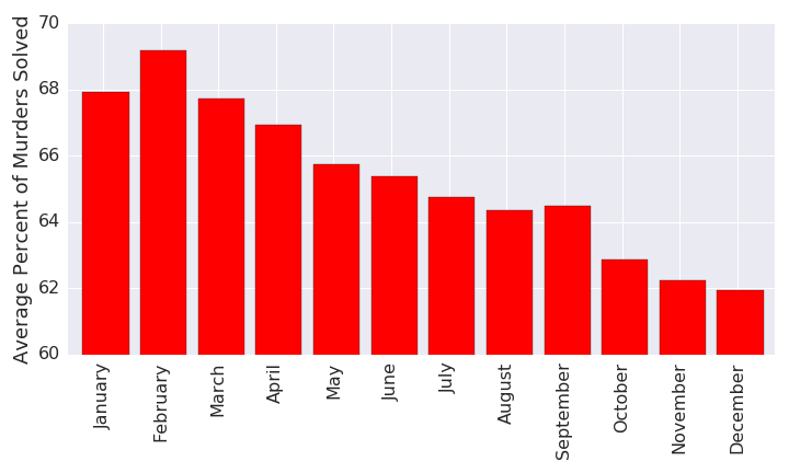
- Very clearly, we see that gun murders are solved less and less as time goes on. That is, as a nation, our accuracy at closing a gun violence case deteriorates as the year progresses.
- Interestingly, we see that the month with the fewest gun murders, February, is also the one with the highest percentage of gun murders solved, at around 69%.
- Another surprising fact is that after December, when the least proportion of crimes are solved, only around 62% nationwide, the solved rate in January jumps up to 68%, that is around 6% within the span of a month! This might be due to many reasons. Perhaps in the December holiday season there is less manpower to spare in solving crimes. Perhaps the surplus of crimes we see in December just swamps police departments at the end of the year. Perhaps the new year in January brings better policies or just work ethic.
- Still it says something as a nation that the percentage of crimes that get solved is nearly monotonically decreasing throughout a given year.
Which States are Best at Solving Murders?
Now that we have looked at crime solving accuracy through time, let us look at it by geography. We all have preconceptions about which states might have the most prevalent issues with gun violence. For example, it is often thought that gun violence is a problem in large metropolitan cities such as Los Angeles, Chicago, and New York City. The extent of this idea remains to be determined by the data but it will help to direct our search in the below map by looking at the containing states: California, Illinois, and New York. We again restrict our dataset to 2000 and beyond to analyze recent trends.
Zoom, pan, click, drag, go nuts with the map below! Clicking on the red diamonds will display the accuracy in solving gun murders since 1980 for each state.
There is obviously a lot of information contained here so let’s just look at one trend, the one we alluded to with states with large metropolitan cities. Looking at New York, we see by its color that only around 50% of gun murders are solved in the state and furthermore this has been the general trend over time. Looking at neighboring Vermont, we see that 90% or more of gun murders are solved. Looking at neighboring Pennsylvania, we see this figure is around 80%.
That is to say, geography may not be the sole factor in why gun murder solve rates are so low in New York. We see a similar story in Illinois, with only around 30% of murders solved in recent years! Compare that to neighboring Indiana at 70% or Iowa at 90%. We see this story repeated in California with only around 50% of gun murders solved in recent years. As comparison, neighboring states such as Nevada seem to be around 80% and Oregon around 90%.
All this is to say, there seems to be some trend between states with big cities (New York City, Los Angeles, and Chicago are the biggest cities by population in the U.S.) and the rate at which gun murders are solved. This is likely attributed to the fact that it is just more difficult to solve crimes in extremely urbanized areas.
And a few other takeaways:
- We see that there is though some geographic clustering of gun murder solve rates, regions where the shading is similar. For example, we see that the Bible Belt, consisting of states like Texas, Arkansas, and Mississippi have rates around 85%. Also, we see that the mountain states including Montana, Idaho, and Wyoming have very high rates around 90%.
- We need to be careful at times when we see a state that is very green. We might assume at first that this state is just really good at solving gun related murders, but often this might not be case. Look at South Dakota for example. Clicking on its red diamond, we see that there are several years where the gun murder solve rate was not just high but at exactly 100%! How can this be? After checking the data, we find that in 2010 for example, there were only 8 gun murders in the entire state of South Dakota. Compare this with a comparably sized state, Delaware, where there were 41 gun murders in 2010. Thus, the authorities in South Dakota need only to solve these 8 murders in order to reach 100% accuracy. Keep this in mind when scanning the map.
Which Cities are Getting Better at Solving Murders?
Even though a state in general might not have a very high accuracy in solving gun murders, it is entirely possible and probable that certain counties in that state are actually quite good at solving gun murders. This might be for various reasons such as regional difference in policing strategies, how well funded certain regions are, or just that there are not many murders in a certain region and so there are less cases to work on at once.
We will explore this idea using the following process. For each state, we will analyze how much better (or worse) that state has gotten in solving gun murders over time. This essentially amounts to computing the slope of the line of best fit in each of the state plots displayed in the above map. For each county in that state, we do the exact same thing.
We then compare all the counties to the state and pick out the county which is improving the most in solving gun murders relative to the state and the county that is deteriorating the most relative to the state. We do this for all states and then pick out the 9 best and 9 worst counties, displayed below. Note that we only consider a county if more than 200 gun murders occurred there since 1980 since we don’t want that problem of having only 2 murders in the county in a given year, for example.
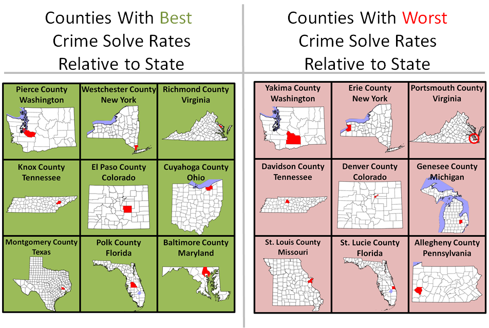
On the left we have the counties that are improving a lot more relative to their states in terms of solving gun murders and on the right we have those counties that are deteriorating considerably worse than their states in solving gun murders.
- We see interestingly that six of the nine states displayed are common between the left and right charts. This intuitively says that these states host counties which are very much extremes in both directions. That is, they host counties that are improving much more than the state, and deteriorating much more than the state.
- One interesting point to note is that for Washington, the most improving county in terms of solved gun murders, Pierce, is directly adjacent to the most deteriorating county, Yakima.
This author could not resist and had to look up demographic information about these two counties in Washington. It turns out that Pierce County is 74.2% white and those of Hispanic or Latino origin made up 9.2% of the population. Yakima County is 63.7% white and those of Hispanic or Latino origin made up 45.0% of the population. There are surely other differences as well, but it is interesting to note the ethnic and racial differences in neighboring counties and how their murder solve rates correlate with that. (Side note: ‘race’ is defined separate from ‘ethnicity’ in the data. ‘White’ falls under race while ‘Hispanic or Latino’ falls under ethnicity and the two are not mutually exclusive.)
This discussion serves as a nice transition to our analysis of disparities in solving crimes by race.
Does Victim Race Affect Whether a Murder is Solved?
One of the most important questions when it comes to what percent of gun murders get solved in a particular state is whether this is dependent at all on whether the victim of the murder was White or Black or Asian or Native American, etc. That is, are there inherent biases in our criminal justice system when it comes to prioritizing a case based on a victim’s race?
It is really important to note here that we will find that quite often that there are disparities in how often gun murders get solved based on victim race, but we need to do more work to figure out exactly why that is.
One easy way we can measure racial disparities in percent of gun murders solved by race is by computing, for a specific state, the percent of gun murders solved for Whites, then for Blacks, then for Asians, then for Native Americans, etc, and then taking the standard deviation of this list. For those unfamiliar with the standard deviation, it measures how much the elements of a list vary from each other.
This is an adept measure here since in a ‘perfect’ world, all races would have their gun murders solved in equal proportions, no racial bias at all. (In a a truly perfect world people wouldn’t choose to kill other people in the first place.) But in our real world, we will see that indeed the percent of gun murders solved does vary by race in each state and the higher the standard deviation, the more these percentages vary and the higher the degree of disparity in that state.
We again limit our search to only year 2000 and later. We also only consider a state if there are three or more racial groups who have 10 or more victims in our 2000-2014 time frame. This is to avoid the issue of a particular state having for example only two Asian victims in that time frame, not a large enough sample size for meaningful comparison. We impose an additional restriction that a state must have at least 150 murders total in that time frame to maintain a meaningful sample size. This is why you might not see each of the 50 states in the chart below.
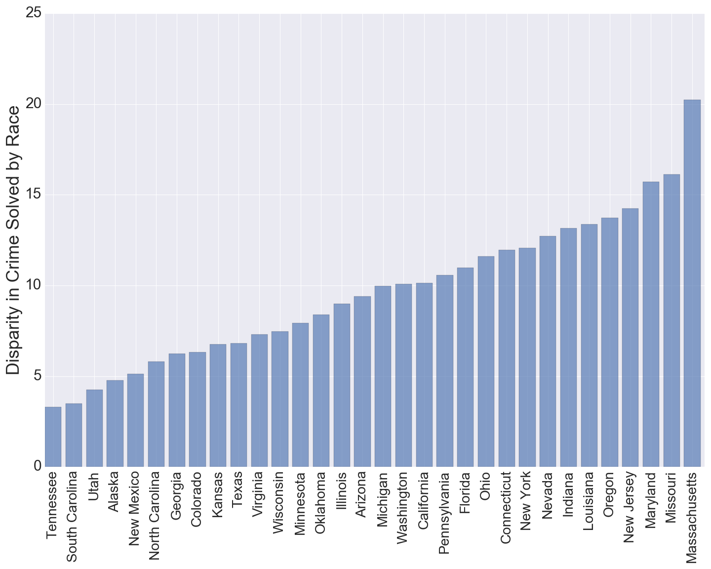
- We see that the disparity level increases gradually for the most part except for at the end with the large jump from Missouri to Massachusetts.
- We see that Tennessee has the lowest disparity of the displayed states and Massachusetts has the highest. It will be interesting to see for these two states exactly what percent of gun murders are solved per each race.
Proportion of Gun Murders Solved by Race in Tennessee vs. Massachusetts
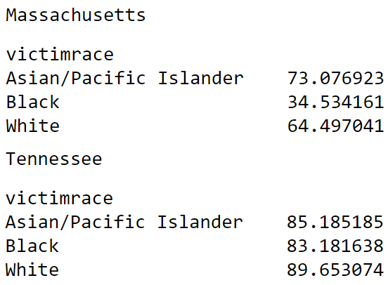
From the output above, we see that the proportions for Tennessee favor clearly Whites and perhaps Asian/Pacific Islanders over Blacks but the numbers are much more equal than those from Massachusetts. We see that in Massachusetts only 34.5% of gun murders are solved for Blacks while that number is 64.5% for Whites, and 73.1% for Asian/Pacific Islanders, more than twice as high as that of Blacks! Clearly this is not just by chance and there is some mechanism in Massachusetts, perhaps as a whole or in certain parts, which drives these greatly disproportionate murder solve rates. This is a good direction for future analysis.
Racial Disparities in Gun Murder Solved through Time
What if we don’t limit our search starting in 2000? Just as we looked at racial biases in space, that is in different U.S. states, what if we want to know how racial disparities in solving gun murders has changed through time, starting in 1980? We can just apply the same methodology to each month from 1980 to 2014, and draw a plot of racial disparity, measured by standard deviation.
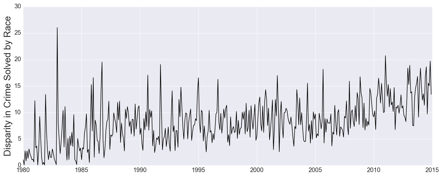
This is not good news. Our plot tells us that racial disparity in gun murder solved has not only been increasing in America since 1980, but it has been doing so in an almost predictable and linear way. Even just looking at recent years, in 2000, the disparity rate was at 8% whereas now it is almost double that around 15%. Why might this be? Are we just getting more racist as a nation? It will be helpful to consider our own national biases but first let’s consider a more fundamental explanation.
The racial composition of the U.S. has changed a lot since 1980. For example, the proportion of the population that is Asian/Pacific Islander or Native American has significantly risen over time. When there are more racial groups, disparity as we measure it is almost expected to rise in the short run due to the low sample size of some racial groups.
Still, we can only use that excuse for so long and even in very recent years, like 2010 until now, when the racial composition has not changed as much as in previous years, we still see the disparity rising linearly as it did since 1980. This trend is indeed worrying. Will it only continue to rise? Or can we somehow reverse it?
Can We Predict the Age of a Killer?
We have been focusing for a long time on which gun murders are solved because of the fundamental fact that there are so many of them that are just never solved: 35% of gun murders in the U.S. since 2000 were not classified as solved. Is there anything we can do as statisticians and data scientists to help out here? If we find ourselves with no information about the killer, can we use predictive analytics to predict their attributes? Another great question is “should we”? Ethics break!
If we are somehow able to use information about a murder such as location, time of day, victim information, weapon type, etc. to predict the race of a killer with high accuracy, should we use this system? For some the answer may be “Yes! Of course! It will help us to catch killers!” For others it may be “No! This just opens the door for data driven racial profiling!” For many more it may be somewhere in between. Post your thoughts in the comments below!
We will be using techniques in machine learning to predict a killer’s age rather than race for this portion of the post. We will be using a more coarse grained approach where we predict not exactly age, but age range. That is, we split up ages into 10 buckets: 0-10 years old, 10-20 years old, …, 90-100 years old, and try to predict which bucket the killer falls into. We use predictors such as month, county, state, murder weapon, victim age, victim race, and victim sex.
We use a classifier called a One-vs-Rest Classifier that trains one model per age bucket and uses those 10 models to make an overall prediction about which age buckets are most likely.
We consider only the gun murders in our data for which the perpetrator was identified and use this subset to train and test our classifiers. We show the result of the prediction for ten randomly chosen perpetrators in the heatmap below. The darker the color (and the higher the number) the more strongly the model thinks the perpetrator’s age is in that bucket. The red outlined squares show the true age bucket.
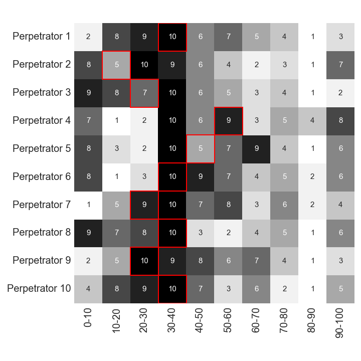
- First off, before even looking at how often we are getting the age bucket right, we see that the most predicted bucket by far is the 30-40 age range. This makes sense since the mean value of perpetrator age (for those solved murders where we actually have this value), is 30.7 years. Thus, the classifier can do well by predicting around the mean value when other information is note useful.
- Looking now at how often the red square matches up with the best prediction, the darkest 10 square, we see it happens 5 out of 10 times in our heatmap. We also are able to match red squares to two 9’s indicating that our second best guess was correct twice. We also see some not so good guesses such as with Perpetrators 2 and 5 where the correct age bucket was not even predicted in the top five guesses.
Overall, our model has an accuracy of 40%, whereas random guessing gets us only 25%, so we get a 15% improvement in predicting the age bucket of the perpetrator using this model. Also, for perpetrators in the 30-40 age range, our model has an accuracy of 38% while random guessing here gets us only 22%, so in this bucket we have actually a 16% increase. Of course, as is evident from the heatmap, the model will rarely pick a perpetrator age bucket of 10-20 or 80-90 and so will miss the few perpetrators that actually fall into such buckets.
Still, with no leads, such a model can give us a start towards finding a killer.
How about Predicting Whether a Crime will be Solved or Not?
Let’s keep the machine learning train going and try now to predict whether or not a gun murder will be solved. We use all the same predictors as in the last machine learning problem: county, state, month, victim information, and weapon used. We restrict our data to only 2014 gun murders to remove the effects of year. We use a classifier called the Random Forest Classifier mainly for its interpretability going forward. In essence, this classifier is structured like a tree which starts at the root and asks a series of yes or no questions about each murder that gives progressively more information about the likely outcome of whether it will be solved or not. For example, it might ask questions like: “Was the victim female?”, “Was the victim under 35 years old?”, “Did this take place in Ohio?”, etc.
The purpose of making this prediction at all is really to understand the relative importance of each predictor in the final prediction. We are interested in knowing things like whether the murder taking place in California gives more information than whether the victim was Black? Does the fact that a handgun was used give more information than the fact that it took place in Chicago? Etc. We can judge the relative importance of a feature by how early on in the tree the question is asked.
After running our model, we find that these are our predictor importances, also called feature importances in machine learning jargon.
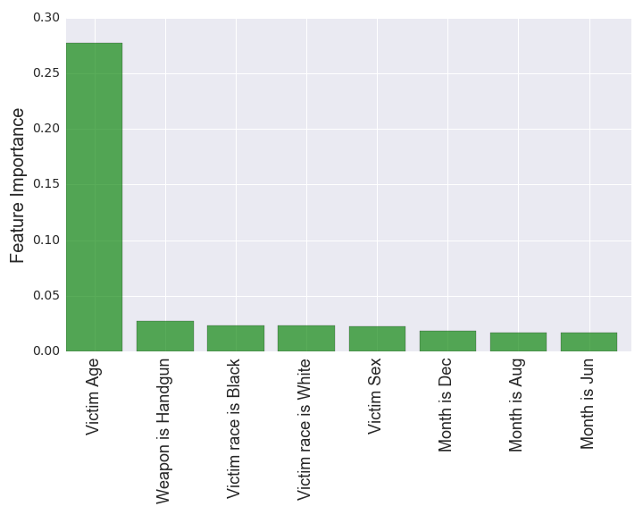
- It is immediately clear that one feature dominates the rest, victim age. Probing the data, we find that the relationship is a positive one. That is, a gun murder is more likely to be solved the older the victim is.
- Aside from this feature, the other top features seem to be on the same scale. Note also that victim age is the only continuous (non-binary) feature in this list. We see that the exact type of gun used, here a handgun, gives us extra information in predicting the fate of the murder. This is likely because, as evidenced by the data, murders committed with handguns are more likely to be solved, but the root cause behind this is likely due to deeper factors about which killers use handguns.
- Interestingly, we see that the next two features are whether the victim is Black or White, respectively. We already have seen evidence of why these are potentially useful features. That is, as we saw with Massachusetts, the solve rate for Blacks tends to be lower or sometimes much lower than that of Whites (nationally and over all time 74% of gun murders were solved for White victims and 64% of gun murders were solved for Black victims). This information implies that it helps to have the victim age when predicting the status of the murder.
- We haven’t talked much about victim sex, but to quickly note: 82% of gun murders where the victim was female are solved while the statistic for gun murders with a male victim is 66% solved. Note also that in 84% of all gun murders the victim was male and only in 16% was the victim female.
- Lastly, looking at the final few features, we see that the month being December gives us the most information out of all other months in determining whether the gun murder will be solved. This is in line with our previous observation that December is the month with the fewest solved gun murders in percentage terms. If we know the crime happened in December, we can more accurately say that it will not be solved.
Ok cool! But, we didn’t see any features relating to geography, state or county, on that list. Where are they? It turns out they appear lower on the list, but we can still glean useful information if we extract only state feature importances and rank them from highest to lowest and do the same for county feature importances. Let’s turn to the state ones first.
Note that the length of the bars are proportional to the relative importance of that state feature.
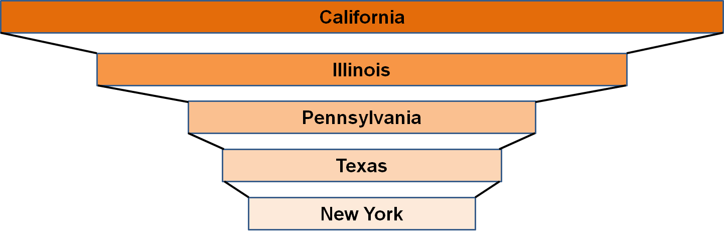
- Perhaps not surprisingly California, home of Los Angeles, and Illinois, home of Chicago, are the best predictors of whether or not a gun murder will be solved. Looking back at our U.S. map, we recall that in recent years, the solve rate in Chicago has been around only 30%, so that if we know a crime occurred there, it helps us to classify it as probably not solved.
Let’s look at counties now.
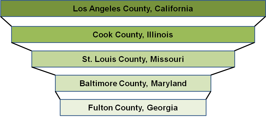
- Again, not surprisingly, especially given the last figure, we see that Los Angeles and Chicago (contained in Cook County) hold the top two spots in determining whether a gun murder will be solved. Indeed, this figure gives us some confirmation that the importances of California and Illinois might be largely driven by these two principal cities respectively.
- We see also on this list Baltimore and St. Louis, often considered some of America’s more “dangerous cities” in terms of murder and violent crime.
Conclusions
So what does it all mean? Should we take all this information and use it to promote gun controls or relax them? Really, whether you are a proponent or opponent of gun controls, we are all, as human beings and Americans, sick and tired of seeing gun murders occur week after week, month after month, year after year. Ending gun violence is a cause we can all get behind.
While our long term goal should be to develop public policy that saves the most Americans from gun related deaths, our immediate goal needs to include a deep and thoughtful analysis about who in our society suffers most from the gun epidemic? Which groups are disproportionately killed by guns and furthermore, for which groups are their murders often left unsolved? We saw in our analysis that gun murders for Blacks are solved at an often sickeningly lower rate than those of Whites. But why? Why does this group often not get the luxury of a closed case? We need a more careful analysis. Attributing it to racial bias in America is a start, but still is not enough as there might be other, related, factors at play we have yet to unearth.
We also need to figure out where we were as a nation and where we are going. As we saw, racial bias in solving gun murders has been almost perfectly linearly increasing over time. As noted, some of this might be because our racial composition as a nation has diversified since 1980, and so mathematically more racial groups will lead to more inequality in the short run. Still, we need to think hard about how to reverse this worrying trend in the long run.
Finally, as new science and new mathematical methods become available, we should absolutely employ them in the realm of predictive policing. The methods outlined here are informative but admittedly basic to what many police departments around the nation are already using. Still, as discussed in the ethics break, we must always be careful about understanding exactly what our model is doing, its own biases, and limitations. Otherwise, we are only transferring bias from humans to machines, and given the high and often blind level of trust people place in statistics and mathematics, this might impede a brighter future.

References
Information on Pierce, Washington
Information on Yakima, Washington
Racial Composition in the U.S. Through Time
Thanks for reading and please leave comments!